In the field of Machine Learning, the practitioner has to work (numerically) with random variables. It is therefore natural to wonder how to sample from a random variable with a computer.

To put it in a nutshell: How to handle randomness with computers?

Syllabus

This tutorial has three main parts.

Random Number Generation

• Handle randomness with a computer
• Understand reproducibility in numerical probability
• Implement your own random number generator. Simulate a lot of probability distributions!

Hands on Statistics

• Compute the expected value of a random variable
• Compute the standard deviation and quantiles of a random variable
• Visualize the weak and strong law of large numbers

Markov Reward Process

• Understand what a Markov Reward Process is
• Simulate Random Walk and Brownian Motion
• Compute the value function of a Markov Reward Process

All code snippets can be copied using the button.

The github repository is

Feel free to use it in order to raise an issue about this post or open the discussion about any related topic.

We start by importing a few necessary libraries, modules and functions.

import numpy as np
from scipy.special import erfinv
import math
import matplotlib.pyplot as plt

Part 1 - Random Number Generation

The main purpose of this part is to raise awareness of the importance of reproducibility as well as teach a (random) bit about algorithmic random number generation.

Please ponder over the following question before delving into the practical: How would you generate a random sequence of numbers?

Can you even think of a high level definition of what it means for a sequence of numbers to be random or random enough?

In machine learning, we deal with random numbers and we need an efficient way to generate random numbers according to some probability distribution. We say that we need a way to simulate the law of a random variable. On the other hand, there is a huge need for reproducibility of the experiments. Reproducibility is a major principle of the scientific method and machine learning (or statistical learning) is no exception. In algorithmic (apart from the very specific field of quantum computing) there is no reason we shouldn’t be able to reproduce exactly an experiment. Therefore, we want to generate random numbers as well as control how those numbers are generated so that we can reproduce computer experiments in pseudo-stochastic environment.

At first glance, reproducibility and randomness may seem like opposite goals.

An algorithm that generates random numbers is called a random number generator and the initial input to this algorithm that allows reproducibility is called the seed.

Question 1

Using numpy, generate two random numbers between 0 and 1 by calling the function np.random.rand. What is different compared to other function calls (e.g. np.sqrt(2))?

# Don't know something? Ask questions on the github repo or read the doc!
?np.random.rand

Answer 1

print(f"Calling np.random.rand(1) twice.\n\
np.random.rand(1) = {np.random.rand(1)}\nnp.random.rand(1) = {np.random.rand(1)}")

print(f"\nCalling np.sqrt(2) twice.\n\
np.sqrt(2) = {np.sqrt(2)}\nnp.sqrt(2) = {np.sqrt(2)}")

Calling np.random.rand(1) twice.
np.random.rand(1) = [0.49799233]
np.random.rand(1) = [0.75253602]

Calling np.sqrt(2) twice.
np.sqrt(2) = 1.4142135623730951
np.sqrt(2) = 1.4142135623730951

What may be surprising (or not, if your are used to it) is that two calls of the same function lead to two different answers (seemingly with the same argument).

At a high level, if we assume that the process that generates thr outputs of successive calls to np.random.rand is deterministic, then the so called initial condition should be enough to completly describe the generated sequence. If the process is complex enough, it may appear random while being completly determnistic and fully described by the generation process and initial condition.

For random number generation, this initial condition is called the seed.

Question 2

The previous question enlightens the fact that there is a need to set the seed so that we can start over a random experiment. We could use np.random.seed to specify a global seed but this is not the recommended way.

The preferred best practice for getting reproducible pseudorandom numbers is to instantiate a generator object with a seed and pass it around. The implicit global RandomState behind the numpy.random. convenience functions can cause problems, especially when threads or other forms of concurrency are involved. Global state is always problematic. We categorically recommend avoiding using the convenience functions when reproducibility is involved. —Robert Kern, NEP 19

Use np.random.default_rng to instanciate a random number generator, generate some random numbers and prove yourself that you know how to start over the generation by generating the same (first) random numbers.

Answer 2

seed = int("ThisIsTheStartOfTheSchoolYear", base=36)%2**31
rng = np.random.default_rng(seed)

print(f"Calling np.random.rand(1) twice.\n\
np.random.rand(1) = {np.random.rand(1)}\nnp.random.rand(1) = {np.random.rand(1)}")

print()
print(f"Calling rng.random(1) twice.\n\
rng.random(1) = {rng.random(1)}\nrng.random(1) = {rng.random(1)}")

Calling np.random.rand(1) twice.
np.random.rand(1) = [0.73463129]
np.random.rand(1) = [0.50966735]

Calling rng.random(1) twice.
rng.random(1) = [0.55043942]
rng.random(1) = [0.18440082]

We start over by feeding the same seed to np.random.default_rng.

seed = int("ThisIsTheStartOfTheSchoolYear", base=36)%2**31
rng = np.random.default_rng(seed)

print(f"Calling np.random.rand(1) twice.\n\
np.random.rand(1) = {np.random.rand(1)}\nnp.random.rand(1) = {np.random.rand(1)}")

print()
print(f"Calling rng.random(1) twice.\n\
rng.random(1) = {rng.random(1)}\nrng.random(1) = {rng.random(1)}")

Calling np.random.rand(1) twice.
np.random.rand(1) = [0.86537091]
np.random.rand(1) = [0.96680284]

Calling rng.random(1) twice.
rng.random(1) = [0.55043942]
rng.random(1) = [0.18440082]

Our own random number generator (in \(]0,1[\))

In the next question, you will implement a Linear Congruential random number generator. Such a rng (random number generator) works as follow. Given an initial integer \(x_0 \in (\underline{M}, \overline{M})\) and an integer function

we generate a sequence of integers by repeatedly applying the function \(f\):

Given \(x_n \in \mathbb{N}\), we can map this integer to a rational \(u_n \in \mathbb{Q} \cap ]0,1[\) by computing

This procedure allows to generate a sequence \((u_n)_n\) of numbers in \(]0,1[\). If the function \(f\) is well chosen, then the sequence \((u_n)_n\) may appear like a sampling from a uniform distribution in \(]0,1[\) (this has a precise mathematical meaning in the field that study this topic).

For mathematical reason, we avoid the value \(0\) and we therefore skip it in any algorithm that implements a rng in the aformentionned fashion. That is to say, if \(x_n = 0\) then set \(x_n\) to \(f(0)\). Therefore, \(f(0)\) should not be equal to \(0\).

Remark: skipping \(0\) may be a property of the rng or a property of the function that calls the rng. In the following, we make it a property of the rng.

The Linear Congruential random number generator (LC-rng) is a function \(f\) of the form \(f(x) = mx + c \hspace{0.3cm} [q]\), that is to say,

Question 3

Implement a class, LC_RNG, that takes a seed (\(x_0\)) as an input and is able to generate a random sequence of numbers in \(]0, 1[\) by calling a random method (it should mimick the behavior of numpy’s).

Use the values \(m = 1103515245\), \(c = 12345\) and \(q = 2^{31}\).

Answer 3

class LC_RNG:
    def __init__(self, seed):
        self.seed = seed
        self.ctr = seed
        
        self.m = 1103515245 
        self.c = 12345
        self.max_int = 2**31
    
    def __str__(self):
        return "Generator (LC_RNG customed)"
    
    def generate_int(self):
        self.ctr = ( self.m * self.ctr + self.c ) % self.max_int
        return self.ctr
        
    def _random(self):
        pseudo_random_int = self.generate_int()
        if pseudo_random_int == 0:
            pseudo_random_int = self.generate_int()
        return pseudo_random_int / self.max_int
    
    def random(self, nbr_samples=None):
        if nbr_samples is None:
            samples = self._random()
        else:
            samples = []
            for _ in range(nbr_samples):
                samples.append(self._random())
        return samples
    
    def normal(self):
        pseudo_random_float = self.random()
        return np.sqrt(2)*erfinv(2*pseudo_random_float-1)

Remember the seed,

seed = int("ThisIsTheStartOfTheSchoolYear", base=36)%2**31

We test our random number generator,

custom_rng = LC_RNG(seed)
print(f"Calling custom_rng.random(1) twice.\n\
custom_rng.random(1) = {custom_rng.random(1)}\ncustom_rng.random(1) = {custom_rng.random(1)}")

Calling custom_rng.random(1) twice.
custom_rng.random(1) = [0.26866815984249115]
custom_rng.random(1) = [0.2322915312834084]

Resetting the seed will restart the same generating process.

custom_rng = LC_RNG(seed)
print(f"Calling custom_rng.random(1) twice.\n\
custom_rng.random(1) = {custom_rng.random(1)}\ncustom_rng.random(1) = {custom_rng.random(1)}")

Calling custom_rng.random(1) twice.
custom_rng.random(1) = [0.26866815984249115]
custom_rng.random(1) = [0.2322915312834084]

This kind of algorithm allows us to generate a random sequence of float in the bounded interval \(]0, 1[\) that is approximately uniformly distributed on this support. From now on, we shall assume in all simulations that the samples from np.random.default_rng are independently and identically distributed according to a uniform distribution in \(]0,1[\).

Question 4

What is the name of the generator that is used by the default call to np.random.default_rng?

Answer 4

What kind of generator is used by default? We can find out by reading the doctstring ?np.random.default_rng (or help(np.random.default_rng) ) or simply using print on the created object. As we can see, this is PCG64.

?np.random.default_rng
print(rng)

Generator(PCG64)

Question 5

Using np.random.default_rng, generate a sequence of 10 000 samples in \(]0,1[\) and plot a histogram. Do the same with your custom rng, LC_RNG.

Answer 5

To compute a histogram, one must arbitrarily partition the segment \(]0,1[\) into sub-interval whose union is the whole segement. In this case, partioning can be seen as a discretization of the probability density function (often abbreviated pdf) with respect to the Lebesgue measure. In computer science, a sub-segment of this sub-division is called a bin.

A histogram is computed by counting the number of samples belonging to each bin. Those counts can be scaled by a common factor afterward. If the scaling factor is such that the sum of the value associated to bins is equal to \(1\), we talk about normalization. In this case, the histogram can be seen as a probability density function with respect to a discrete measure. This last remark is a bit advanced and you can pursue your reading even without understanding it, as long as you have an intuition of what a histogram represent.

plt.figure(figsize=(11,5))
plt.title(f"Density histogram of 10 000 samples generated by np.random.default_rng with the seed {seed}")
plt.hist([rng.random() for _ in range(10000)], density=True, bins=50)
plt.show()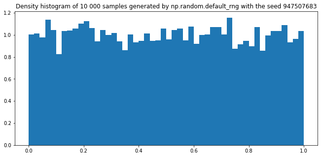

plt.figure(figsize=(11,5))
plt.title(f"Density histogram of 10 000 samples generated by custom_rng with the seed {seed}")
plt.hist([custom_rng.random() for _ in range(10000)], density=True, bins=50)
plt.show()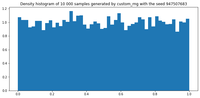

Generating/Simulating a random variables

Theorem (Inverse Transform Sampling) Let $U$ be a uniform random variable on \(]0,1[\) and \(X\) a real random variable. Assume that the cumulative distribution function \(F_X\) of \(X\), \(F_X (u) = \mathbb{P} (X \leq u)\), is continuous. Then the random variable \(Y\),

has distribution \(F_X\). That is to say, \(X\) and \(Y\) have the same law .

An algorithmic consequence of this theorem is that to generate (or simulate) i.i.d. samples having the law of a random variable \(X\), one can first use a generator of uniform samples in \(]0,1[\) and then use the inverse distribution function \(F_X^{-1}\) to compute i.i.d. samples from \(X\).

Of course, such a method assumes that we have a way to compute (or estimate with good enough precision) \(F_X^{-1}\).

Algorithm for generating a sample from random variable X using \(F_X^{-1}\)

• Generate u uniformly at random on \(]0,1[\)
• Output \(F_x^{-1}(u)\)

The function \(F_X^{-1}\) of a unitary centered Normal distribution (a.k.a. Gaussian), \(X \sim \mathcal{N}(0,1)\), is implemented in the next cell.

# Gaussian distribution
F_gaussian_inv = lambda u : np.sqrt(2)*erfinv(2*u-1)

N = 5000
x = np.linspace(0+1e-5, 1-1e-5, N)
y = F_gaussian_inv(x)
plt.figure(figsize=(9,5))
plt.title("Invert distribution function of a unitary centered gaussian random variable")
plt.plot(x,y)
plt.show()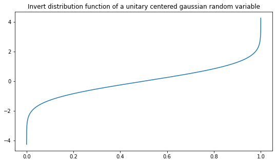

Question 6

Using np.random.default_rng, generate a sequence of 10 000 samples according to a unitary centered gaussian distribution and plot a histogram. Modify the LC_RNG to do the same with your custom rng.

Answer 6

Simulation using numpy random number generator

plt.figure(figsize=(9,5))
plt.title(f"Density histogram of 10 000 samples generated by np.random.default_rng with the seed {seed} (gaussian)")
plt.hist(rng.normal(size=10000), density=True, bins=50)
plt.show()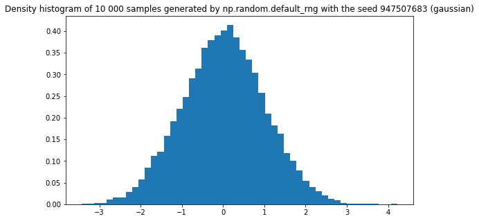

Simulation using custom random number generator

We add the _normal and normal methods to our LC_RNG class.

class LC_RNG:
    def __init__(self, seed):
        self.seed = seed
        self.ctr = seed
        
        self.m = 1103515245 
        self.c = 12345
        self.max_int = 2**31
    
    def __str__(self):
        return "Generator (LCG customed)"
    
    def generate_int(self):
        self.ctr = ( self.m * self.ctr + self.c ) % self.max_int
        return self.ctr
        
    def _random(self):
        pseudo_random_int = self.generate_int()
        if pseudo_random_int == 0:
            pseudo_random_int = self.generate_int()
        return pseudo_random_int / self.max_int
    
    def random(self, nbr_samples=None):
        if nbr_samples is None:
            samples = self._random()
        else:
            samples = []
            for _ in range(nbr_samples):
                samples.append(self._random())
        return samples
    
    def _normal(self):
        pseudo_random_float = self.random()
        return np.sqrt(2)*erfinv(2*pseudo_random_float-1)
    
    def normal(self, nbr_samples=None):
        if nbr_samples is None:
            samples = self._normal()
        else:
            samples = []
            for _ in range(nbr_samples):
                samples.append(self._normal())
        return samples
    
custom_rng = LC_RNG(seed)

plt.figure(figsize=(9,5))
plt.title(f"Density histogram of 10 000 samples generated by custom_rng with the seed {seed} (gaussian)")
plt.hist(custom_rng.normal(10000), density=True, bins=50)
plt.show()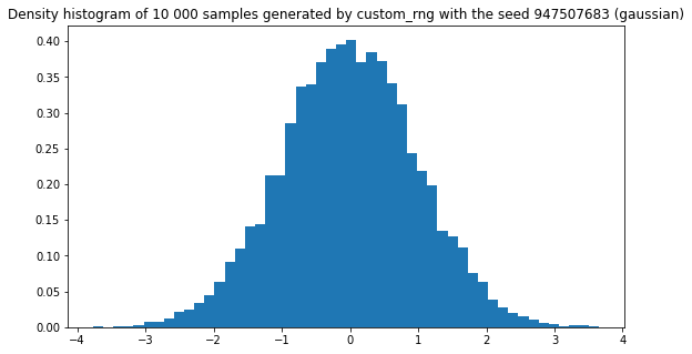

Great! Everything is visually pleasing! It seems to work! Yeah sure, but…

Question 7

What could have gone wrong? Implement a Dummy_LC_RNG class with \(c=1\) and \(m=128\). Re-do the previous experiments and try changing m from 128 to 127 and see what happens.

Answer 7

First with \(m = 128\).

class Dummy_LC_RNG:
    def __init__(self, seed, m=128):
        self.seed = seed
        self.ctr = seed
        
        self.m = m
        self.c = 1
        self.max_int = 2**31
    
    def __str__(self):
        return "Dummy Generator (LCG customed)"
    
    def generate_int(self):
        self.ctr = ( self.m * self.ctr + self.c ) % self.max_int
        return self.ctr
        
    def random(self):
        pseudo_random_int = self.generate_int()
        if pseudo_random_int == 0:
            pseudo_random_int = self.generate_int()
        return pseudo_random_int / self.max_int

dummy_rng = Dummy_LC_RNG(seed)
plt.figure(figsize=(9,5))
plt.hist([dummy_rng.random() for _ in range(10000)], density=True, bins=50)
plt.show()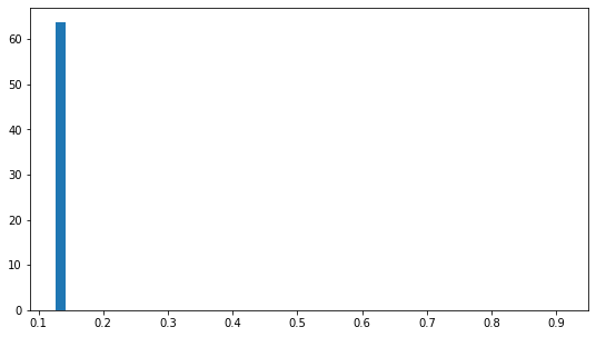

Then with \(m = 127\).

dummy_rng = Dummy_LC_RNG(seed, 127)
plt.figure(figsize=(9,5))
plt.hist([dummy_rng.random() for _ in range(10000)], density=True, bins=50)
plt.show()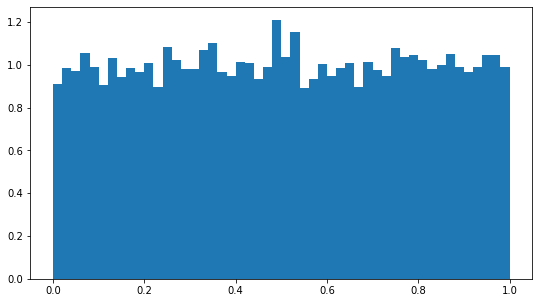

As it can be seen, one must be careful when crafting a pseudo random number generator. Furthermore, one should also be careful that \(x_{n+1}\) and \(x_n\) are as independent as possible. Although this may seem counter-intuitive to do so with a completely deterministic procedure, there are ways to measure the statistical correlation of samples.

An analogy is the one of shuffling a deck of cards. While shuffling is a completely deterministic procedure we have a feeling that after shuffling, if done correctly, we get a random permutation of the cards that is roughly independent from the original permutation of the deck before shuffling.

Part 2 - Hands on Statistics

In this part, we show how to compute the expected value of a sequence of numbers, or of a random variable that we can simulate. In both cases, the practionaer has access to a stream of numbers generated by a possibly unknown and possibly random process.

Expected value is a mathematical way of answering the question: What’s happening on average?

For instance, what is

• the average temperature in your city
• the average temperature in your city during winter
• the average height of trees
• the average time in air when a human is jumping
• The average number brain consumption of \(O_2\) when answering a maths question
• …

It is often a first step into the modelisation or despcription of a system, albeit a coarse description. Later in this tutorial, we will see how to compute the standard deviation, a measure of dispersion around the average value.

Compared to the median, another mathematical notion of average, the expected value is easier to compute on a sequential fashion.

There are two main ways to compute the mean of a sequence of numbers, an offline and an online way. Given a sequence \((x_i)_{i \in \{1, \cdots , n \}}\) of real numbers, we can compute the mean \(\bar x_n\) by first computing the sum of all the elements, \(\sum_i x_i\) and then dividing by the number of elements. This is the offline method. If we were given a new number \(x_{n+1}\) we would have to re-do all the additions and division. Mathematically, the formula is:

The online way computes a sequence of means, \((\bar x_k)_{k \in \{1, \cdots , n \} }\), where \(\bar x_k\) is the mean of the subsequence (or slice) \((x_i)_{i \in \{1, \cdots , k \}}\). The last element of the sequence of means is the mean of the original sequence. Mathematically, we initiate the sequence with \(\bar x_1 = x_1\) and the update rule is:

The advantage of the online method is that we don’t need to store the sequence of all samples and that we can immediatly update the mean once given a new sample.

Question 8

Check that the online methods indeed is correct.

Answer 8

A proof can by made by induction with initial condition \(\bar x_1 = x_1\) and following induction step

Question 9

Write as many functions as you can to compute the mean of a python list and check on a random sequence if they give the same result. What can you say?

Answer 9

def mean_1(l):
    agg = 0
    i = 0
    for elm in l:
        agg += elm
        i += 1
    return agg / i

def mean_2(l):
    m = 0
    i = 0
    for elm in l:
        m = (i*m + elm)/(i+1)
        i += 1
    return m

def mean_3(l):
    m = np.sum(l) / len(l)
    return m

def mean_4(l):
    m = sum(l) / len(l)
    return m

def mean_5(l):
    m = math.fsum(l) / len(l)
    return m

samples = rng.random(1000)
print(f"mean_1(samples)  = {mean_1(samples)}\n\
mean_2(samples)  = {mean_2(samples)}\n\
mean_3(samples)  = {mean_3(samples)} (same result than np.mean)\n\
mean_4(samples)  = {mean_4(samples)}\n\
mean_5(samples)  = {mean_5(samples)}\n\
np.mean(samples) = {np.mean(samples)} (float64)\n\
np.mean(samples) = {np.mean(samples, dtype='float32')} (float32)\n\
np.mean(samples) = {np.mean(samples, dtype='float16')}  (float16)\n")

mean_1(samples)  = 0.5103409440103216
mean_2(samples)  = 0.5103409440103205
mean_3(samples)  = 0.5103409440103216 (same result than np.mean)
mean_4(samples)  = 0.5103409440103216
mean_5(samples)  = 0.5103409440103216
np.mean(samples) = 0.5103409440103216 (float64)
np.mean(samples) = 0.5103409290313721 (float32)
np.mean(samples) = 0.51025390625  (float16)

Depending on the implementation, and the arithmetic precision used, we get differents results. Those differences are mainly due to how arithmetic precision is handled and the order in which we perform the operation. Even if some operations are associative in a mathematical way (on the paper), those may not be in floating point arithmetic due to the very finite nature of numerical computation. In floating point arithmetic \((a + b) + c \neq a + (b + c)\), see accuracy problems.

Below, we emphasize this fact by testing different ways of summing elements of a list.

def sum_1(l):
    agg = 0
    for elm in l:
        agg += elm
    return agg

def sum_3(l):
    m = np.sum(l)
    return m

def sum_4(l):
    m = sum(l)
    return m

def sum_5(l):
    m = math.fsum(l)
    return m

print(f"sum_1(samples)  = {sum_1(samples)}\n\
sum_3(samples)  = {sum_3(samples)} (same result than np.mean)\n\
sum_4(samples)  = {sum_4(samples)}\n\
sum_5(samples)  = {sum_5(samples)}\n\
np.sum(samples) = {np.sum(samples)} (float64)\n\
np.sum(samples) = {np.sum(samples, dtype='float32')} (float32)\n\
np.sum(samples) = {np.sum(samples, dtype='float16')}  (float16)\n")

sum_1(samples)  = 510.34094401032155
sum_3(samples)  = 510.34094401032155 (same result than np.mean)
sum_4(samples)  = 510.34094401032155
sum_5(samples)  = 510.3409440103216
np.sum(samples) = 510.34094401032155 (float64)
np.sum(samples) = 510.3409423828125 (float32)
np.sum(samples) = 510.25  (float16)

Question 10

Let \((X_i)_{i \in \{1, \cdots , n\}}\) be \(n\) i.i.d. random variables such that \(X_i \sim X\) with \(\mathbb{E}(X) = \mu\).

The Law of large numbers states that the empirical mean of those \(n\) i.i.d. random variables,

converges (in some sense) to \(\mu\) as \(n\) tends to infinity.

Write an experiment that collects 10 000 samples from a unitary centered gaussian distribution, and computes the sequence of updated means. Plot the histogram of samples (as above) and the function \(k \mapsto \bar x_k\).

Answer 10

class experiment:
    def __init__(self, nbr_samples=0, mean=0):
        assert nbr_samples >= 0
        self.nbr_samples = nbr_samples
        self.mean = mean
        
        # We store information, only for the plots
        self.samples = []
        self.means = []
    
    def update_mean(self, elm):
        self.mean = (self.nbr_samples * self.mean + elm) / (self.nbr_samples+1)
        self.nbr_samples += 1
        
        # Storage for the plots
        self.means.append(self.mean)
        self.samples.append(elm)

xp = experiment()

nbr_experiments = 1000
for _ in range(nbr_experiments):
    sample = rng.normal()
    xp.update_mean(sample)

plt.figure(figsize=(9,5))
plt.title("Samples repartition")
plt.hist(xp.samples, density=True, bins=50)
plt.show()

plt.figure(figsize=(9,5))
plt.title("Mean estimation as a function of the number of samples")
plt.plot(xp.means)
plt.show()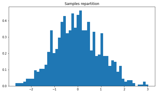

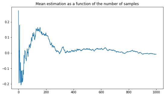
It is quite interesting to see this random nature of the expected value, yet to know that in the long run, it will be close to the true average. In the next question, this random behavior is highlighted by plotting several trajectories. At the same time, the convergence of those plot to the same value emphasizes some regularity in this random behavior. Some of this regularity is clarified by the central limit theorem.

Question 11

Repeat 10 times the experiments of the previous question and plot the 10 trajectories \(k \mapsto \bar x_k\). Add the curves \(k \mapsto \pm \frac{1}{\sqrt{k}}\) to your plot. Comment if you remember the central limit theorem, otherwise, come back with the next question in hindsight.

Answer 11

nbr_experiments = 10
nbr_samples = 500
plt.figure(figsize=(9,5))
plt.title("Mean estimation as a function of the number of samples")
for _ in range(nbr_experiments):
    xp = experiment()
    for _ in range(nbr_samples):
        sample = rng.normal()
        xp.update_mean(sample)
    plt.plot(xp.means)

plt.plot([1/np.sqrt(n) for n in range(1, 501)], linewidth=2.5, c='black', linestyle='--')
plt.plot([-1/np.sqrt(n) for n in range(1, 501)], linewidth=2.5, c='black', linestyle='--')

plt.show()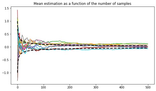

By plotting more trajectories and removing the first initials time steps, one can better visualize the asymptotic results stated by the central limit theorem: the density of curves at the end point might look like a gaussian random variable.

nbr_experiments = 50
nbr_samples = 500
plt.figure(figsize=(9,5))
plt.xticks([n for n in range(20, 501,40)])
plt.title("Mean estimation as a function of the number of samples")
for _ in range(nbr_experiments):
    xp = experiment()
    for _ in range(nbr_samples):
        sample = rng.normal()
        xp.update_mean(sample)
    plt.plot([n for n in range(20, 500)], xp.means[20:])
plt.plot([n for n in range(20, 500)], [1/np.sqrt(n) for n in range(21, 501)], linewidth=2.5, c='black', linestyle='--')
plt.plot([n for n in range(20, 500)],[-1/np.sqrt(n) for n in range(21, 501)], linewidth=2.5, c='black', linestyle='--')

plt.show()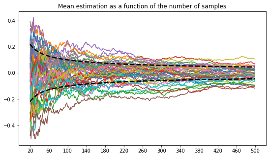

Question 12

Let \((X_i)_{i \in \{1, \cdots , n\}}\) be \(n\) i.i.d. random variables such that \(X_i \sim X\) with \(\mathbb{E}(X) = \mu\) and \(\mathbb{V}(X) = \sigma^2\). The Central Limit Theorem states that the empirical mean of those \(n\) i.i.d. random variables,

has the law of a Gaussian random variable, \(\mathcal{N} (\mu, \frac{\sigma}{\sqrt{n}})\) in the limit of large \(n\).

Let \(X\) be a random variable having the uniform law on \(]0,1[\). Craft an experiment to visualize the central limit theorem when samples are drawn from \(X\).

Answer 12

We sample 300 000 lists of 1000 samples generated according to a uniform law in \(]0,1[\). For each list, we compute the mean and create a list of the 300 000 means. Then we plot a histogram of this list. If 1000 is large enough for the central limit theorem to roughly apply, then the histogram of the list of means resemble the one of a gaussian distribution with mean \(\mu = 0\) and standard deviation \(\sigma = 1/\sqrt{1000} \simeq 0.03\).

nbr_list = 300000
means = []
for _ in range(nbr_list):
    l = rng.random(1000)
    means.append(mean_1(l))

plt.figure(figsize=(11,5))
plt.title("Means repartition")
plt.hist(means, density=True, bins=100)
plt.show()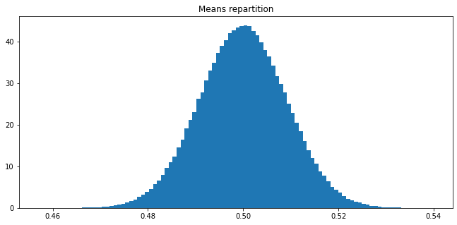

Standard deviation and Quantiles

Given a list of samples drawn from a random variable \(X\), what relevant quantities could be computed? In the previous subsection, we emphasize the empirical mean and illustrate how it is related to the true mean \(\mathbb{E}(X)\). Given the empirical mean, it is natural to measure the spread of the samples around that value. In other words, we want to compute an empirical version of the standard deviation.

There are two main ways of computing the empirical standard deviation. One that is called the uncorrected standard deviation,

and the other that is called the corrected standard deviation

Remark: np.std computes the uncorrected standard deviation.

Intuitively, it corresponds to two viewpoints on how to handle small sample size. When \(n=1\), \(\hat \sigma_u = 0\) while \(\hat \sigma_c = \frac{0}{0}\) i.e., is not defined. Indeed, when \(n=1\), one could think one of the two things

• The empirical standard deviation is 0 since there is no deviation in the dataset
• The empirical standard deviation is undefined since there is no way to empirically compute a deviation in the dataset

On the other hand, \(\hat \sigma_u \rightarrow \sigma\), and \(\hat \sigma_u \rightarrow \sigma\), meaning that both estimators have the same asymptotic behaviors (large sample size). In particular,

Mathematically, \(\hat \sigma_u\) is a biased estimator (\(\mathbb{E}(\hat \sigma_u) \neq \sigma\)) and \(\hat \sigma_c\) is an unbiased estimator (\(\mathbb{E}(\hat \sigma_c) = \sigma\)). Bias is not necessarily a problem because a small bias can sometimes be traded against a reduction in the variance of the estimator (as it is the case here).

Question 13

Implement functions computing the two empirical standard deviation. Check that both numerically converges to \(\sigma\) as the number of samples increases.

Answer 13

samples = custom_rng.normal(500000)

def standard_deviation_uncorrected(samples):
    mu = mean_1(samples)
    std = sum((samples - mu)**2) / len(samples)
    return np.sqrt(std)

def standard_deviation_corrected(samples):
    assert len(samples) > 1, "The length of the samples array should be strictly larger than 1"
    mu = mean_1(samples)
    std = sum((samples - mu)**2) / (len(samples) -1)
    return np.sqrt(std)

print(standard_deviation_uncorrected(samples))
print(standard_deviation_corrected(samples))

1.0006729694819605
1.000673970156431

Another natural way to compute the spread of a list of samples is via a function. This function associates a number \(F(x)\) to each interval \([\mu - x, \mu + x]\) with \(x>0\); \(F(x)\) is the fraction of samples that lies within it. In particular, it is interesting to know the fraction of samples lying in \([\mu - \sigma, \mu + \sigma]\).

For the readers aware of the notion, this is highly related to the concept of cumulative distribution function.

plt.figure(figsize=(9,5))
plt.title(f"Density histogram of samples generated according a Gaussian distribution")
plt.hist(samples, density=True, bins=80)
s = standard_deviation_corrected(samples)
m = mean_1(samples)
plt.arrow(m-s, 0.2, 2*s, 0, head_length=0, head_width=0, width=0.007, shape="full", fc="black", ec="black")
plt.text(m, 0.22, "$\mu\pm\sigma$", ha='center', va='center', color="black", size=20)

plt.arrow(m-2*s, 0.15, 4*s, 0, head_length=0, head_width=0, width=0.007, shape="full", fc="red", ec="red")
plt.text(m, 0.17, "$\mu\pm2\sigma$", ha='center', va='center', color="red", size=20)

plt.arrow(m-3*s, 0.1, 6*s, 0, head_length=0, head_width=0, width=0.007, shape="full", fc="pink", ec="pink")
plt.text(m, 0.12, "$\mu\pm3\sigma$", ha='center', va='center', color="pink", size=20)
plt.show()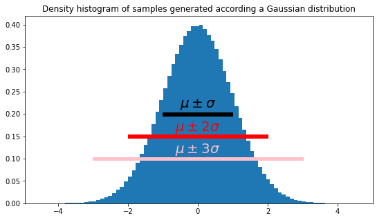

Question 14

What percentage of samples fall in the interval \([\mu - \sigma, \mu+\sigma]\)? and \([\hat\mu - \hat\sigma, \hat\mu+\hat\sigma]\)? Check the 68-95–99.7 rule.

Answer 14

def percent(samples, sigma=1, mu=0):
    ctr = 0
    for sample in samples:
        if sample >= mu - sigma and sample <= mu + sigma:
            ctr += 1
    return ctr / len(samples)

print(percent(samples, 1)*100)
print(percent(samples, 2)*100)
print(percent(samples, 3)*100)

68.22240000000001
95.41460000000001
99.72800000000001

Question 15

Implement a function that computes the \(\alpha\) quantile of a list of samples, that is to say, an empirical value \(\hat x_\alpha\) that corresponds to the true value \(x_\alpha\), defined as

Using this function, how can you compute the median? How is the median different from the mean?

Answer 15

def quantile(samples, alpha):
    sorted_samples = np.sort(samples)
    k = np.floor(alpha*len(samples))
    return samples[k]

To compute the empirical median, one can use the quantile function to compute \(\hat x_{1/2}\).

Part 3 - Markov Reward Process

In the following, we consider sequences of random variables that are not necessarily i.i.d. That is, we will introduce a dependency model in the sequence of random variables. In the i.i.d. case, the index \(n \in \mathbb{N}\) of an element \(X_n\) of the sequence of random variables is somewhat arbitrary. It is mainly a way of pointing to an object in a collection. In the following, we introduce a type of dependency that is called Markovian and makes use of the order \(\leq\) of the natural number \(\mathbb{N}\). The element of the sequence are seen as if they were generated in order and the index n is often thought of as time. However, keep in mind that the Markov property can be extended beyond sequences indexed by natural number or ordered set. For instance, Markov random field are indexed by elements of topological space and neighborhoods give a dependency relation between the elements of the collection.

Back to where we were, we want to study sequences represented as

In the following, we shall assume that the generative process is Markovian, i.e., the future is independent from the past given the present. The sequence may therefore be represented as

where \(p\) is called the probability transition function. In the following, this function is independent of \(n\) (time homogeneity property). Therefore, the model may be represented more concisely:

together with an initial distribution of \(X_0\).

Question 16

Consider the Markov chain

where \(X_0 = 0\) and

Write a fonction that generate a sequence of \(n\) samples according to this process. Plot such a trajectory. Zoom-in. What can you say?

Answer 16

def random_walk(horizon):
    start = 0
    values = [0]
    for _ in range(horizon):
        x = rng.random()
        if x < 0.5:
            values.append(values[-1] + 1)
        else:
            values.append(values[-1] - 1)
    return values

H = 10000
rw = random_walk(H)

plt.figure(figsize=(9,5))
plt.title("1D random walk")
plt.xlabel("time steps")
plt.ylabel("value")
plt.plot(rw)
plt.show()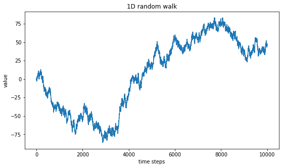

An educated eye may see some auto-similarity pattern in the generated curve. That is to say, a similar pattern (made of up-and-down sharp wave) seems to be spotten at diffent scales. To investigate this property, we “zoom-in” by plotting only the curve between the times steps 4000 and 6000 instead of the whole 10 000 time steps represented above.

plt.figure(figsize=(9,5))
plt.title("1D random walk - zooming in")
plt.xlabel("time steps")
plt.ylabel("value")
plt.plot(range(4000,6000),rw[4000:6000])
plt.show()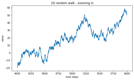

One can see that zooming-in does not really change the type of curve that we had at a larger scale. It is only when we zoom-in even further that we can start to see the characteristic length of 1 introduced by our generating method, \(X_{n+1} = X_n \pm 1\). Below, we zoom-in on 500 time steps only. Of course, another characteristic length is playing a role here, which is also equal to 1 and corresponds to the distance between two consecutive time steps.

plt.figure(figsize=(9,5))
plt.title("1D random walk - zooming in")
plt.xlabel("time steps")
plt.ylabel("value")
plt.plot(range(4000,4500),rw[4000:4500])
plt.show()

Discretized Brownian motion

Question 17

Answer the same question than the previous one but with a process such that \(X_{n+1} \mid X_n \sim \mathcal{N}(X_n, \epsilon)\). That is to say,

where \((G_n^{\epsilon})_{n\in\mathbb{N}}\) is a sequence of i.i.d. gaussian random variable with the law \(\mathcal{N}(0,\epsilon)\).

Answer 17

Intuitively, we should obtain a “similar” type of curve with a characteristic length of \(\epsilon\). However, because this process can take its values in \(\mathbb{R}\) rather than \(\mathbb{N}\) only, the characteristic time discretization will play a more important role in the viualizations of the plots.

def brownian_motion(horizon, epsilon=0.1):
    start = 0
    values = [0]
    for _ in range(horizon):
        x = rng.normal()
        values.append(values[-1] + epsilon*x)
    return values

H = 10000
bm = brownian_motion(H)

plt.figure(figsize=(9,5))
plt.title("1D Brownian motion")
plt.xlabel("time steps")
plt.ylabel("value")
plt.plot(bm)
plt.show()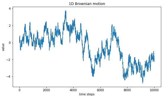

Indeed, we see the same auto-similar pattern and can try to zoom-in to better visualize this pattern.

plt.figure(figsize=(9,5))
plt.title("1D random walk - zooming in")
plt.xlabel("time steps")
plt.ylabel("value")
plt.plot(range(4000,6000),bm[4000:6000])
plt.show()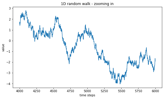

Question 18

Write a function that computes and plots a discretized Brownian motion in 2D.

Answer 18

def brownian_motion2d(horizon, epsilon=0.1):
    start = 0
    X = [0]
    Y = [0]
    for _ in range(horizon):
        x = rng.normal()
        y = rng.normal()
        X.append(X[-1] + epsilon*x)
        Y.append(Y[-1] + epsilon*y)
    return X,Y

H = 10000
X, Y = brownian_motion2d(H)

plt.figure(figsize=(9,9))
plt.title("2D Brownian motion")
plt.xlabel("x")
plt.ylabel("y")
plt.plot(X, Y, alpha=0.7)
plt.show()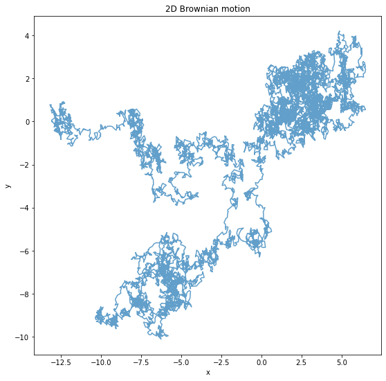

plt.figure(figsize=(9,9))
plt.title("2D Brownian motion - zooming in")
plt.xlabel("x")
plt.ylabel("y")
plt.plot(X[5000:7000], Y[5000:7000], alpha=0.7)
plt.show()

plt.figure(figsize=(9,9))
plt.title("2D Brownian motion - several trajectories")
plt.xlabel("x")
plt.ylabel("y")
for _ in range(10):
    X, Y = brownian_motion2d(H)
    plt.plot(X, Y, alpha=0.7)
plt.show()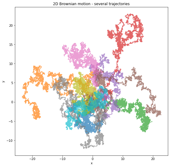

Random walk on a graph

In the following, we will consider random walks on a graph where the set of vertices \(V\) is finite as well as the set of edges \(E\). At each vertex \(v \in V\) is attached a probability distribution \(p_v\) on the space of vertices such that \(p_v (n)\) is probability of going from vertex \(v\) to vertex \(n\). In the Markov reward process litterature, a vertex is often called a state.

The specificity of Markov reward process is that a reward \(r\) function assign a number to each transition (or step). Formally, at each state \(v \in V\), \(r_v\) is a function that assign a reward \(r_v(n)\) to each transition from state \(v\) to state \(n\).

To create a random walk on a graph, one first create a graph with weighted edges. Using those weight, we create a transition distribution at each vertex. Using the following code as a starting point, this is the topic of the next question.

import networkx as nx

plt.figure(figsize=(11,11))
Graph = nx.gnp_random_graph(10, 0.5, directed=True)
nx.draw(Graph, with_labels=True, node_color='green')
plt.show()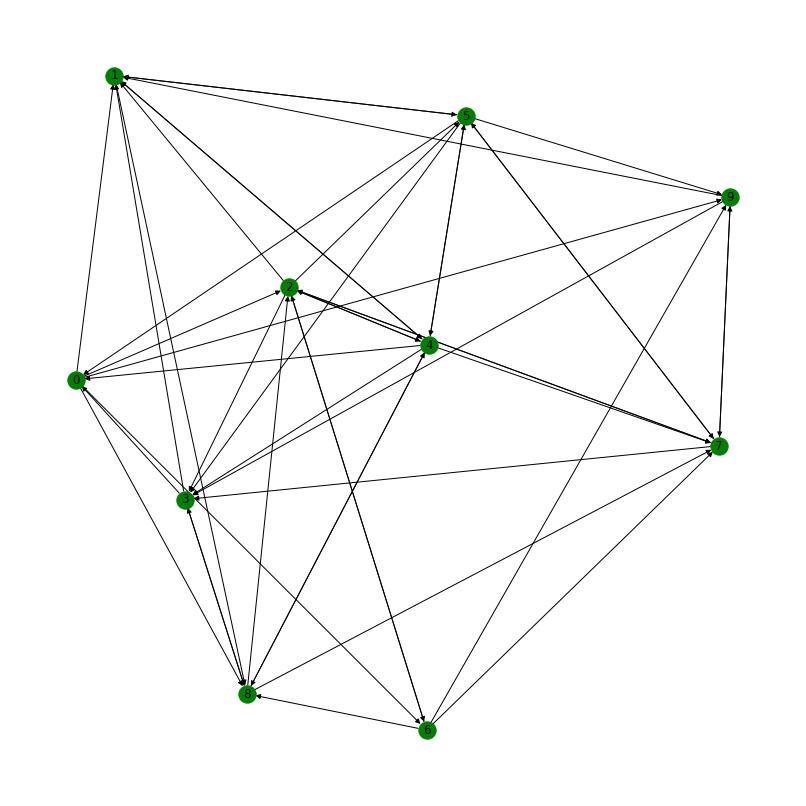

for (u,v,w) in Graph.edges(data=True):
    w['weight'] = rng.random()
    w['reward'] = rng.normal() + 2

Question 19

Given a labeled directed graph \(G = (V, E, w, r, v_0)\) where \(V\) is the set of vertices, \(E\) the set of edges, \(w: E \rightarrow ]0,1[\) and \(r: E \rightarrow \mathbb{R}\) and \(v_0 \in V\) we can compute a Markovian random walk on the vertices of \(G\) by considering that

The specificity of this random walk is that at each transition \(v_{i-1} \rightarrow v_i\), we collect a reward \(r(v_{i-1}, v_i)\).

Write a function that generates a random walk along a graph, collects the history of vertices (i.e. samples) and collects the history of rewards. Plot the updated mean reward (it should be around 2, but why?).

Answer 19

def random_walk_graph(G, horizon=1000, starting_node=0):
    samples = []
    nodes = [starting_node]
    for _ in range(horizon):
        adj_data = G.adj[nodes[-1]]
        neighbors = []
        weights = []
        for n in adj_data:
            neighbors.append(n)
            weights.append(adj_data[n]['weight'])
        w = sum(weights)
        proba = [h/w for h in weights]
        next_node = np.random.choice(neighbors, p=proba)
        nodes.append(next_node)
        samples.append(adj_data[next_node]['reward'])
    return nodes, samples

nodes, rewards = random_walk_graph(Graph)
mean_reward = np.cumsum(rewards)/np.arange(1,len(rewards)+1)

plt.figure(figsize=(9,5))
plt.title("Mean cumulative reward gathered along random walk on a graph")
plt.xlabel("time steps")
plt.ylabel("value")
plt.plot(mean_reward)
plt.show()

Because all edges have an associated reward that is initially generated according to a gaussian distribution with mean 2, we expected the mean cumulative reward collected to be around this value. Of course, previous sections highlighted how the random nature of sampling can generate dispersion around the mean.

Doing more experiments.

Below, we generate 10 graphs and for each one, compute the mean cumulative reward curve. We see that those curves all seem to converge and that those limit are gathered around 2 as we should expect.

plt.figure(figsize=(9,5))
plt.title("Mean cumulative reward gathered along random walk on a graph")
plt.xlabel("time steps")
plt.ylabel("value")
for _ in range(10):
    for (u,v,w) in Graph.edges(data=True):
        w['weight'] = rng.random()
        w['reward'] = rng.normal() + 2
    nodes, rewards = random_walk_graph(Graph)
    mean_reward = np.cumsum(rewards)/np.arange(1,len(rewards)+1)
    plt.plot(mean_reward)
plt.show()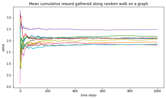

To wrap it up, we generate gain 10 random graphs and for each one, compute the mean cumulative reward curve. We see that those curves all seem to converge and that those limit are gathered around 5 as we should expect. Why?

plt.figure(figsize=(9,5))
plt.title("Mean cumulative reward gathered along random walk on a graph")
plt.xlabel("time steps")
plt.ylabel("value")
for _ in range(10):
    for (u,v,w) in Graph.edges(data=True):
        w['weight'] = rng.random()
        w['reward'] = rng.normal() + 10*rng.random()
    nodes, rewards = random_walk_graph(Graph, horizon=100)
    mean_reward = np.cumsum(rewards)/np.arange(1,len(rewards)+1)
    plt.plot(mean_reward)
plt.show()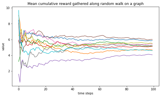

Experiment and play with those models! If you have any remarks or questions, feel free to reach me, my door is always open!